Hard mode
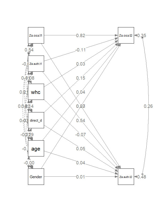
First do a normal plot, then one with nodeLabels then order vars in a grid and display with that layout
Step 1:
fit.l.ao <- sem(l.ao, data=dat, estimator ="MLM", std.lv=TRUE)
semPaths(fit.l.ao, style="lisrel", layout="tree", whatLabels= "std", nCharNodes = 0, edge.label.cex= 1,
  label.cex=1, sizeMan = 8, sizeLat = 8, rotation=2)

Step 2:
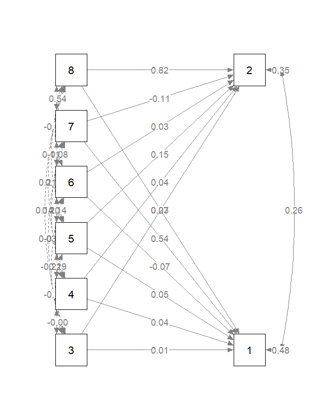
fit.l.ao <- sem(l.ao, data=dat, estimator ="MLM", std.lv=TRUE)
semPaths(fit.l.ao, style="lisrel", layout="tree", whatLabels= "std", nCharNodes = 0, edge.label.cex= 1,
  label.cex=1, sizeMan = 8, sizeLat = 8, nodeLabels = 1:8, rotation=2)

Step 3:
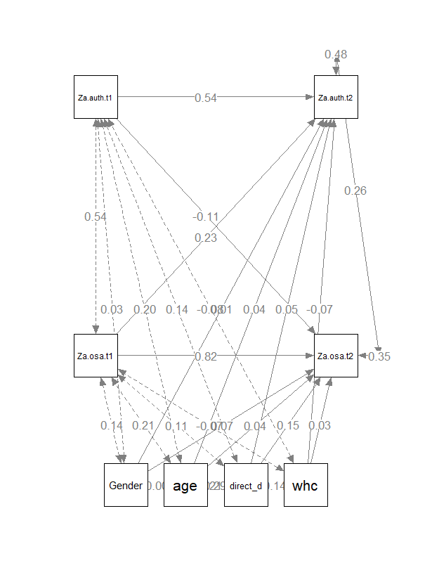
#arrange vars in a grid matrix
x=c(3,1,0,0,0,0,3,1)
y=c(5,5,-2,0,2,4,-3,-3)
ly=matrix(c(y,x), ncol=2)
# plot the result
semPaths(fit.l.ao, style="lisrel", layout=ly, whatLabels= "std", nCharNodes = 0, edge.label.cex= 1,
         label.cex=1, sizeMan = 8, sizeLat = 8, rotation=2,edge.label.position=0.45)

This format is for sure not perfect. You can specify everything… but it is a lot of work
Easy mode
I found a better approach to quickly plot models. First, specify what nodes to keep. This makes it way easier to see what’s going on.
# only keep those vars
test <- semptools::keep_nodes(
  semPlotModel(mal2),
  c("al", "batl", "aut", "com", "rel", "mot"))

# specify a grid of vars. They will be presented in this grid row, col, use the actual
# var names in the latent model. var 1 is the first var that is defined in the model
lmt <- layout_matrix(al = c(2, 1),
                     aut = c(1, 2),
                     com = c(2, 2),
                     rel = c(3, 2),
                     mot = c(1, 3),
                     btl = c(3, 3))

# plot the model
s <- semPaths(test, whatLabels="std", style="ram", residuals=FALSE, label.scale=TRUE,
         edge.label.cex=2, rotation=2, layout=lmt, edge.label.position=0.45)
Add significance signs
Also, you can add sig. signs which is very helpful.
# use these signs
alsi <- c(`†` = 0.1, `*` = 0.05, `**` = 0.01, `***` = 0.001)

# update the plot
s2 <- mark_sig(s, test, alphas = alsi)
plot(s2)