Table of contents

Load packages
Basic example
Second example
Power analysis

Load packages

library(lme4)
library(tidyverse)
library(afex)
library(summarytools)
library(performance)
library(MASS)
library(DescTools)
library(sjPlot)

Basic example

Intercept-Only Model

This is a df with students nested within classrooms Intercept only model estimates the grand mean of the response across all occasions and individuals. This is the baseline / null model.

m0 <- lmer(popular ~ 1 + (1 | l2id), data=df)
summary(m0)

## Linear mixed model fit by REML. t-tests use Satterthwaite's method [
## lmerModLmerTest]
## Formula: popular ~ 1 + (1 | l2id)
##    Data: df
## 
## REML criterion at convergence: 6330.5
## 
## Scaled residuals: 
##     Min      1Q  Median      3Q     Max 
## -3.5655 -0.6975  0.0020  0.6758  3.3175 
## 
## Random effects:
##  Groups   Name        Variance Std.Dev.
##  l2id     (Intercept) 0.7021   0.8379  
##  Residual             1.2218   1.1053  
## Number of obs: 2000, groups:  l2id, 100
## 
## Fixed effects:
##             Estimate Std. Error       df t value Pr(>|t|)    
## (Intercept)  5.07786    0.08739 98.90973    58.1   <2e-16 ***
## ---
## Signif. codes:  0 '***' 0.001 '**' 0.01 '*' 0.05 '.' 0.1 ' ' 1

5.07786*** sig. random intercept.
This refers to the expected value (i.e., average) popularity in students in all classrooms (classroom grand mean for popularity).
0.7021 is the classroom variation in popularity.
1.2218 is the individual level variation in popularity.

Note. I am using lmeTest which uses denominator degrees of freedom. P values in multi level modeling is questionable. Other p values are possible. e.g., with the “KR” Kenward-Roger approximation for degrees of freedom. This can be done with the library(afex)

ICC

performance::icc(m0)

## # Intraclass Correlation Coefficient
## 
##     Adjusted ICC: 0.365
##   Unadjusted ICC: 0.365

We can also calculate icc by hand:

0.7021 /(1.2218 + 0.7021)

## [1] 0.3649358

This icc justifies investigating multi-level modeling. This means that 36% of the variation in the popularity comes from the variation of classrooms.

This means that 64% is due to individual characteristics of students.
Another way to think about this is that if you randomly select two students from the same classroom the expected correlation in their popularity rating is 36%!

A different way is to look at ranova from the lmerTest package and see if p is significant.
Here p is sig. indicating sig. variation of intercepts, justifying clustering with mlm.
The intercepts are unconditional classroom means here

ranova(m0)

## ANOVA-like table for random-effects: Single term deletions
## 
## Model:
## popular ~ (1 | l2id)
##            npar  logLik    AIC LRT Df Pr(>Chisq)    
## <none>        3 -3165.3 6336.5                      
## (1 | l2id)    2 -3487.8 6979.5 645  1  < 2.2e-16 ***
## ---
## Signif. codes:  0 '***' 0.001 '**' 0.01 '*' 0.05 '.' 0.1 ' ' 1

Add some predictors

m1 <- lmer(popular ~ 1 + texp + sex + (1 | l2id), data=df)
summary(m1)

## Linear mixed model fit by REML. t-tests use Satterthwaite's method [
## lmerModLmerTest]
## Formula: popular ~ 1 + texp + sex + (1 | l2id)
##    Data: df
## 
## REML criterion at convergence: 5544
## 
## Scaled residuals: 
##     Min      1Q  Median      3Q     Max 
## -3.6546 -0.6520  0.0012  0.6721  3.1327 
## 
## Random effects:
##  Groups   Name        Variance Std.Dev.
##  l2id     (Intercept) 0.3606   0.6005  
##  Residual             0.8307   0.9114  
## Number of obs: 2000, groups:  l2id, 100
## 
## Fixed effects:
##              Estimate Std. Error        df t value Pr(>|t|)    
## (Intercept) 3.621e+00  1.530e-01 1.004e+02  23.666  < 2e-16 ***
## texp        5.406e-02  9.655e-03 9.774e+01   5.599 1.98e-07 ***
## sex         1.351e+00  4.395e-02 1.957e+03  30.732  < 2e-16 ***
## ---
## Signif. codes:  0 '***' 0.001 '**' 0.01 '*' 0.05 '.' 0.1 ' ' 1
## 
## Correlation of Fixed Effects:
##      (Intr) texp  
## texp -0.898       
## sex  -0.122 -0.026

anova(m0,m1)

## refitting model(s) with ML (instead of REML)

## Data: df
## Models:
## m0: popular ~ 1 + (1 | l2id)
## m1: popular ~ 1 + texp + sex + (1 | l2id)
##    npar    AIC    BIC  logLik deviance  Chisq Df Pr(>Chisq)    
## m0    3 6333.5 6350.3 -3163.7   6327.5                         
## m1    5 5538.5 5566.5 -2764.2   5528.5 799.01  2  < 2.2e-16 ***
## ---
## Signif. codes:  0 '***' 0.001 '**' 0.01 '*' 0.05 '.' 0.1 ' ' 1

Second example

Study design

The example data is from (Brown & Strand, 2019) and I heavily follow instructions form Schad (2019) and Brown (2021).

The example study is a within-subjects speech-perception study. 53 participants were presented 553 isolated words.

Conditions:

The auditory modality alone (0; audio-only condition) OR with an accompanying video of the talker (1; audiovisual condition).
Participants listened to and repeated these isolated words aloud while simultaneously performing an unrelated response time task in the tactile modality.
Participants identified speech in both an easy (0) and a hard (1) level of background noise.

Describe hypotheses

h1: Modality affects response time. h2: the effect of modality on response time depends on (i.e., interacts with) the level of the background noise

Import dataset

dat <- read_csv("rt_dummy_data_interaction.csv")

Screening

head(dat)

## # A tibble: 6 x 5
##     PID    RT SNR   modality   stim 
##   <dbl> <dbl> <chr> <chr>      <chr>
## 1   301  1024 Easy  Audio-only gown 
## 2   301   838 Easy  Audio-only might
## 3   301  1060 Easy  Audio-only fern 
## 4   301   882 Easy  Audio-only vane 
## 5   301   971 Easy  Audio-only pup  
## 6   301  1064 Easy  Audio-only rise

the dataset is already in the desired format: “unaggregated long format”

each of the first six rows corresponds to a different word (stim) presented to the same participant (PID)

H1: X on Y

Modality affects response time.

Outlier detection

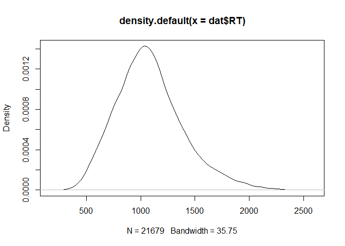
plot(density(dat$RT))

qqnorm(dat$RT)

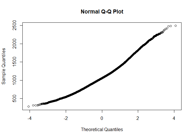
->no outliers

m1 <- lm(RT ~ modality, data = dat)
summary(m1)

## 
## Call:
## lm(formula = RT ~ modality, data = dat)
## 
## Residuals:
##     Min      1Q  Median      3Q     Max 
## -814.52 -210.46  -25.52  174.54 1436.54 
## 
## Coefficients:
##                     Estimate Std. Error t value Pr(>|t|)    
## (Intercept)         1041.464      3.001  347.00   <2e-16 ***
## modalityAudiovisual   83.057      4.207   19.74   <2e-16 ***
## ---
## Signif. codes:  0 '***' 0.001 '**' 0.01 '*' 0.05 '.' 0.1 ' ' 1
## 
## Residual standard error: 309.7 on 21677 degrees of freedom
## Multiple R-squared:  0.01766,    Adjusted R-squared:  0.01761 
## F-statistic: 389.7 on 1 and 21677 DF,  p-value: < 2.2e-16

check_outliers(m1)

## OK: No outliers detected.

->no outliers

Descriptive stats

ggplot(data=dat, aes(x=modality, y=RT)) + geom_boxplot()

dfSummary(dat)

## Data Frame Summary  
## dat  
## Dimensions: 21679 x 5  
## Duplicates: 0  
## 
## -----------------------------------------------------------------------------------------------------------------
## No   Variable      Stats / Values               Freqs (% of Valid)     Graph                 Valid      Missing  
## ---- ------------- ---------------------------- ---------------------- --------------------- ---------- ---------
## 1    PID           Mean (sd) : 332.8 (19.5)     53 distinct values     . .             . :   21679      0        
##      [numeric]     min < med < max:                                    : : . :   : . . : :   (100.0%)   (0.0%)   
##                    301 < 333 < 364                                     : : : : . : : : : :                       
##                    IQR (CV) : 36 (0.1)                                 : : : : : : : : : :                       
##                                                                        : : : : : : : : : :                       
## 
## 2    RT            Mean (sd) : 1083.7 (312.5)   1712 distinct values         :               21679      0        
##      [numeric]     min < med < max:                                        . : .             (100.0%)   (0.0%)   
##                    279 < 1057 < 2488                                       : : :                                 
##                    IQR (CV) : 392 (0.3)                                  . : : : .                               
##                                                                          : : : : : . .                           
## 
## 3    SNR           1. Easy                      11191 (51.6%)          IIIIIIIIII            21679      0        
##      [character]   2. Hard                      10488 (48.4%)          IIIIIIIII             (100.0%)   (0.0%)   
## 
## 4    modality      1. Audio-only                10647 (49.1%)          IIIIIIIII             21679      0        
##      [character]   2. Audiovisual               11032 (50.9%)          IIIIIIIIII            (100.0%)   (0.0%)   
## 
## 5    stim          1. peace                        81 ( 0.4%)                                21679      0        
##      [character]   2. foul                         47 ( 0.2%)                                (100.0%)   (0.0%)   
##                    3. jock                         47 ( 0.2%)                                                    
##                    4. same                         47 ( 0.2%)                                                    
##                    5. hog                          46 ( 0.2%)                                                    
##                    6. late                         46 ( 0.2%)                                                    
##                    7. safe                         46 ( 0.2%)                                                    
##                    8. sham                         46 ( 0.2%)                                                    
##                    9. bear                         45 ( 0.2%)                                                    
##                    10. cage                        45 ( 0.2%)                                                    
##                    [ 533 others ]               21183 (97.7%)          IIIIIIIIIIIIIIIIIII                       
## -----------------------------------------------------------------------------------------------------------------

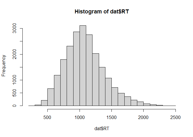
->no missings, we already see RT might not be non-normaly distributed

Normality test

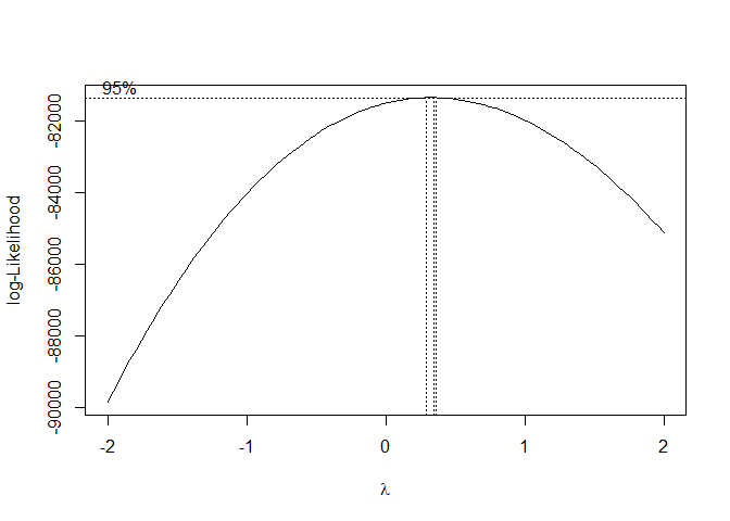
boxcox(m1)

hist(dat$RT)

PlotQQ(dat$RT) 

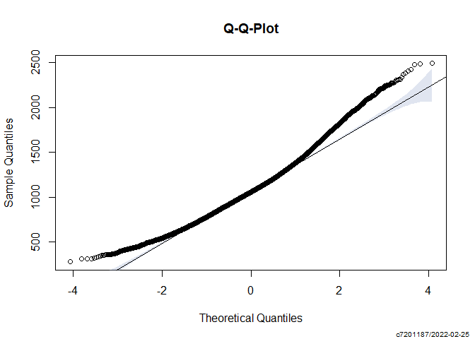
shapiro.test(dat$RT)

Too many samples instead use Anderson-Darling

#install.packages('nortest')
library(nortest)

ad.test(dat$RT)

## 
##  Anderson-Darling normality test
## 
## data:  dat$RT
## A = 91.12, p-value < 2.2e-16

justifiable to transform due to non-normal data. However, Mixed modeling is quite robust to violations of the normality assumption (Brown 2021), so I will continue without transformation.. Still, an argument can be made that this is incorrect

Define contrasts

treatment-coding / dummy coding will be used. the audio-only condition is the reference level; coded as 0, and the audiovisual condition is coded as 1. This has an effect on the intercept of the regression models.

What does this mean for later interpretations?

The regressions intercept of the LMM later represents the estimated mean response time in the audio-only condition (when modality = 0).
The coefficient associated with the effect of modality indicates how the mean response time changes in the audiovisual condition (when modality = 1).
Other contrasts will not change the fit of the model but i change the interpretation of the regression coefficients.

Visualise between participant

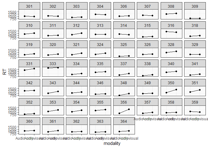
t_dat <- plyr::ddply(dat, c("modality","PID"), summarize, RT=mean(RT))

ggplot(data=t_dat, aes(x=modality, y=RT, group=1)) +
  geom_point() + geom_line() +
  facet_wrap(~PID) + theme(strip.text.x = element_blank()) + theme_bw()

Define & run LMM models

Following Brown I calculate by-participant and by-item random intercepts and slopes! The reason is that both participants and words might differ in the extent to which they are affected by the modality manipulation

In this example participants and words are modeled as random effects because they are randomly sampled from their respective populations, and this accounts for variability within those populations.

modality is modeled as a fixed effect because the common influence of modality on response times across participants and items is modeled.

To model variability between subjects, random slopes are included in the model specification.

audio-only is the reference level

dat$modality <- ifelse(dat$modality == "Audio-only", 0, 1)

Build full model

m2 <- lmer(RT ~ 1 + modality + (1 + modality|PID) + (1 + modality|stim), data = dat)

## Warning in checkConv(attr(opt, "derivs"), opt$par, ctrl = control$checkConv, :
## Model failed to converge with max|grad| = 0.00882975 (tol = 0.002, component 1)

model failed to converge

Deal with non converging models

now I could calculate reduced “maximal models” use Principal Component Analysis etc. One option e.g, is to force the correlations among random effects to be zero and test nested models with and without the variable. To remove a correlator use like this (0 + modality|PID). But sometimes the random-effects structure is too complex (Bates, Kliegl, et al., 2015). There are multiple other options to solve this. “?convergence” might help
Brown(2021) suggests to try the all_fit() function from the afex package to look for an optimizer that works.

all_fit(m2)

## bobyqa. : [OK]
## Nelder_Mead. : [OK]
## optimx.nlminb :

## Lade nötigen Namensraum: optimx

## [ERROR]
## optimx.L-BFGS-B :

## Lade nötigen Namensraum: optimx

## [ERROR]
## nloptwrap.NLOPT_LN_NELDERMEAD :

## Warning in checkConv(attr(opt, "derivs"), opt$par, ctrl = control$checkConv, :
## Model failed to converge with max|grad| = 0.00882975 (tol = 0.002, component 1)

## [OK]
## nloptwrap.NLOPT_LN_BOBYQA :

## Warning in checkConv(attr(opt, "derivs"), opt$par, ctrl = control$checkConv, :
## Model failed to converge with max|grad| = 0.00882975 (tol = 0.002, component 1)

## [OK]
## nmkbw. : [ERROR]

## $bobyqa.
## Linear mixed model fit by REML ['lmerModLmerTest']
## Formula: RT ~ 1 + modality + (1 + modality | PID) + (1 + modality | stim)
##    Data: dat
## REML criterion at convergence: 302385.7
## Random effects:
##  Groups   Name        Std.Dev. Corr 
##  stim     (Intercept)  17.43        
##           modality     14.72   0.16 
##  PID      (Intercept) 168.98        
##           modality     87.81   -0.17
##  Residual             255.46        
## Number of obs: 21679, groups:  stim, 543; PID, 53
## Fixed Effects:
## (Intercept)     modality  
##     1044.14        83.18  
## 
## $Nelder_Mead.
## Linear mixed model fit by REML ['lmerModLmerTest']
## Formula: RT ~ 1 + modality + (1 + modality | PID) + (1 + modality | stim)
##    Data: dat
## REML criterion at convergence: 302385.7
## Random effects:
##  Groups   Name        Std.Dev. Corr 
##  stim     (Intercept)  17.43        
##           modality     14.72   0.16 
##  PID      (Intercept) 168.98        
##           modality     87.81   -0.17
##  Residual             255.46        
## Number of obs: 21679, groups:  stim, 543; PID, 53
## Fixed Effects:
## (Intercept)     modality  
##     1044.14        83.18  
## 
## $optimx.nlminb
## <simpleError in getOptfun(optimizer): "optimx" package must be installed order to use "optimizer=\"optimx\"">
## 
## $`optimx.L-BFGS-B`
## <simpleError in getOptfun(optimizer): "optimx" package must be installed order to use "optimizer=\"optimx\"">
## 
## $nloptwrap.NLOPT_LN_NELDERMEAD
## Linear mixed model fit by REML ['lmerModLmerTest']
## Formula: RT ~ 1 + modality + (1 + modality | PID) + (1 + modality | stim)
##    Data: dat
## REML criterion at convergence: 302385.7
## Random effects:
##  Groups   Name        Std.Dev. Corr 
##  stim     (Intercept)  17.43        
##           modality     14.73   0.16 
##  PID      (Intercept) 169.08        
##           modality     87.80   -0.16
##  Residual             255.46        
## Number of obs: 21679, groups:  stim, 543; PID, 53
## Fixed Effects:
## (Intercept)     modality  
##     1044.14        83.18  
## optimizer (nloptwrap) convergence code: 0 (OK) ; 0 optimizer warnings; 1 lme4 warnings 
## 
## $nloptwrap.NLOPT_LN_BOBYQA
## Linear mixed model fit by REML ['lmerModLmerTest']
## Formula: RT ~ 1 + modality + (1 + modality | PID) + (1 + modality | stim)
##    Data: dat
## REML criterion at convergence: 302385.7
## Random effects:
##  Groups   Name        Std.Dev. Corr 
##  stim     (Intercept)  17.43        
##           modality     14.73   0.16 
##  PID      (Intercept) 169.08        
##           modality     87.80   -0.16
##  Residual             255.46        
## Number of obs: 21679, groups:  stim, 543; PID, 53
## Fixed Effects:
## (Intercept)     modality  
##     1044.14        83.18  
## optimizer (nloptwrap) convergence code: 0 (OK) ; 0 optimizer warnings; 1 lme4 warnings 
## 
## $nmkbw.
## <packageNotFoundError in loadNamespace(x): es gibt kein Paket namens 'dfoptim'>

For example the bobyqa optimizer should work. I suspect this is because of the non normal distribution of RT.
For example: lmer uses the “nloptwrap” optimizer by default; and glmer uses a combination of bobyqa and NelderMead
Py-BOBYQA is a flexible package for finding local solutions to nonlinear, nonconvex minimization problems (with optional bound constraints), without requiring any derivatives of the objective.

lets try with optimizer = “bobyqa”

Compare full model with nested model

m3 <- lmer(RT ~ 1 + modality + 
          (1 + modality|PID) + (1 + modality|stim), 
          data = dat, 
          control = lmerControl(optimizer = "bobyqa"))

->it worked

now compare the model including the effect of interest (e.g., modality) with a model lacking that effect (i.e., a nested model) using a likelihood- ratio test.

m3_re <- lmer(RT ~ 1 + (1 + modality|stim) + (1 + modality|PID), 
                       data = dat, 
                       control = lmerControl(optimizer = "bobyqa"))

Compare nested models

anova(m3_re, m3)

## refitting model(s) with ML (instead of REML)

## Data: dat
## Models:
## m3_re: RT ~ 1 + (1 + modality | stim) + (1 + modality | PID)
## m3: RT ~ 1 + modality + (1 + modality | PID) + (1 + modality | stim)
##       npar    AIC    BIC  logLik deviance  Chisq Df Pr(>Chisq)    
## m3_re    8 302449 302513 -151217   302433                         
## m3       9 302419 302491 -151200   302401 32.385  1  1.264e-08 ***
## ---
## Signif. codes:  0 '***' 0.001 '**' 0.01 '*' 0.05 '.' 0.1 ' ' 1

Chisq = 32.385, Df = 1, p = 1.264e-08
The small p value in the Pr(>Chisq) column indicates that the model including the modality effect provides a better fit for the data than the model without it; thus, the modality effect is significant.

Bonus: to speed up likelihood-ratio tests

These log likelihood-ratio tests are tedious with multiple fixed effects.
afex package speeds up process. Mixed() function takes a model specification as input and conducts likelihood-ratio tests on all fixed (but not random) effects in the model when the argument method = ‘LRT’ is included.
Bonus: you do not see the reduced models that were built to obtain the relevant p values, so the temptation to inadvertently p-hack is reduced.

mixed(RT ~ 1 + modality + 
        (1 + modality|PID) + (1 + modality|stim), 
      data = dat, 
      control = lmerControl(optimizer = "bobyqa"), 
      method = 'LRT')

## Contrasts set to contr.sum for the following variables: stim

## Numerical variables NOT centered on 0: modality
## If in interactions, interpretation of lower order (e.g., main) effects difficult.

## REML argument to lmer() set to FALSE for method = 'PB' or 'LRT'

## Fitting 2 (g)lmer() models:
## [..]

## Mixed Model Anova Table (Type 3 tests, LRT-method)
## 
## Model: RT ~ 1 + modality + (1 + modality | PID) + (1 + modality | stim)
## Data: dat
## Df full model: 9
##     Effect df     Chisq p.value
## 1 modality  1 32.39 ***   <.001
## ---
## Signif. codes:  0 '***' 0.001 '**' 0.01 '*' 0.05 '+' 0.1 ' ' 1

it automatically fits multiple lmer models and compares them with likelihood-ratio tests you get the same results as before X2=32.385 df=1 p=1.264e-08

Investigate efects

summary(m3)

## Linear mixed model fit by REML. t-tests use Satterthwaite's method [
## lmerModLmerTest]
## Formula: RT ~ 1 + modality + (1 + modality | PID) + (1 + modality | stim)
##    Data: dat
## Control: lmerControl(optimizer = "bobyqa")
## 
## REML criterion at convergence: 302385.7
## 
## Scaled residuals: 
##     Min      1Q  Median      3Q     Max 
## -3.3646 -0.6964 -0.0140  0.5886  5.0003 
## 
## Random effects:
##  Groups   Name        Variance Std.Dev. Corr 
##  stim     (Intercept)   303.9   17.43        
##           modality      216.7   14.72   0.16 
##  PID      (Intercept) 28552.7  168.98        
##           modality     7709.8   87.81   -0.17
##  Residual             65258.8  255.46        
## Number of obs: 21679, groups:  stim, 543; PID, 53
## 
## Fixed effects:
##             Estimate Std. Error      df t value Pr(>|t|)    
## (Intercept)  1044.14      23.36   52.14  44.704  < 2e-16 ***
## modality       83.18      12.58   52.09   6.615 2.02e-08 ***
## ---
## Signif. codes:  0 '***' 0.001 '**' 0.01 '*' 0.05 '.' 0.1 ' ' 1
## 
## Correlation of Fixed Effects:
##          (Intr)
## modality -0.178

intercept = 1044.14 this is the mean response time in the dummy 0 group, audio only 83 ms slower in the audiovisual condition.
random effect correlation stim and modality corr = .16 This means that words (stim) that were responded to more slowly in the audio-only condition tended to have larger (more positive, steeper) slopes
random effect correlation PID and modality corr = -.17 participants who responded more slowly in the audio-only condition had shallower slopes.

sanity check

library(psych)

describeBy(dat$RT, dat$modality)

## 
##  Descriptive statistics by group 
## group: 0
##    vars     n    mean     sd median trimmed    mad min  max range skew kurtosis
## X1    1 10647 1041.46 302.42   1013 1023.18 274.28 279 2478  2199 0.64     0.67
##      se
## X1 2.93
## ------------------------------------------------------------ 
## group: 1
##    vars     n    mean     sd median trimmed    mad min  max range skew kurtosis
## X1    1 11032 1124.52 316.56   1100 1107.74 295.04 310 2488  2178 0.56     0.47
##      se
## X1 3.01

Plot effects H1

I only have 1 fixed effect so…

sjPlot::plot_model(m3, 
                   axis.labels=c("modality"),
                   show.values=TRUE, show.p=TRUE,
                   title="Effect of modality on RT")

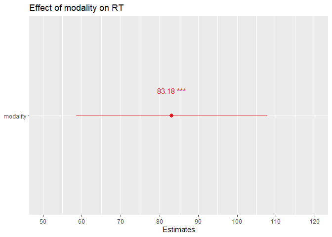
you can report from here, can tweak output

sjPlot:: tab_model(m3)

->this will give a nice table

Describe results

I will copy the results section from Brown(2021)

A likelihood-ratio test indicated that the model including modality provided a better fit for the data than a model without it, χ2(1) = 32.39, p < .001. Examination of the summary output for the full model indicated that response times were on average an estimated 83 ms slower in the audiovisual relative to the audio-only condition(β = 83.18, SE = 12.58, t = 6.62).

H2: Interaction

Define and run model

condition easy (coded 0) and a hard (coded 1) level of background noise

dat$SNR <- ifelse(dat$SNR == "Easy", 0, 1)

the full model did not run removed the correlation between the random intercept for stimulus and the by-stimulus random slope for modality we aren’t actually interested in that correlation

m4 <- lmer(RT ~ 1 + modality + SNR + modality:SNR +
             (0 + modality|stim) + (1|stim) + (1 + modality + SNR|PID), 
           data = dat,
           control = lmerControl(optimizer = 'bobyqa'))
summary(m4)

## Linear mixed model fit by REML. t-tests use Satterthwaite's method [
## lmerModLmerTest]
## Formula: RT ~ 1 + modality + SNR + modality:SNR + (0 + modality | stim) +  
##     (1 | stim) + (1 + modality + SNR | PID)
##    Data: dat
## Control: lmerControl(optimizer = "bobyqa")
## 
## REML criterion at convergence: 301138.2
## 
## Scaled residuals: 
##     Min      1Q  Median      3Q     Max 
## -3.5354 -0.6949 -0.0045  0.5972  4.8706 
## 
## Random effects:
##  Groups   Name        Variance Std.Dev. Corr       
##  stim     modality      144.7   12.03              
##  stim.1   (Intercept)   356.3   18.88              
##  PID      (Intercept) 25522.7  159.76              
##           modality     8044.7   89.69   -0.03      
##           SNR         10355.6  101.76    0.02 -0.47
##  Residual             61234.2  247.46              
## Number of obs: 21679, groups:  stim, 543; PID, 53
## 
## Fixed effects:
##               Estimate Std. Error        df t value Pr(>|t|)    
## (Intercept)    998.824     22.214    52.729  44.964  < 2e-16 ***
## modality        98.510     13.199    59.065   7.464 4.41e-10 ***
## SNR             92.339     14.790    58.004   6.243 5.39e-08 ***
## modality:SNR   -29.532      6.755 21298.850  -4.372 1.24e-05 ***
## ---
## Signif. codes:  0 '***' 0.001 '**' 0.01 '*' 0.05 '.' 0.1 ' ' 1
## 
## Correlation of Fixed Effects:
##             (Intr) modlty SNR   
## modality    -0.063              
## SNR         -0.014 -0.354       
## modalty:SNR  0.074 -0.247 -0.232

intercept represents the estimated response time when all other predictors are set to 0. participants have 998.824 responsetime in easy condition, audio only

Simple effects

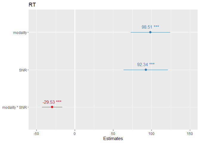
modality coeff = response times are on average 98.510 ms slower in the audio-visual relative to the audio-only condition in the easy listening condition (SNR = 0).
SNR effect indicates that response times are on average 92 ms slower in the hard relative to the easy listening condition, but this applies only when the modality dummy code is set to 0 (representing the audio-only condition).

sjPlot::plot_model(m4, show.values=TRUE, show.p=TRUE,)

tab_model(m4, pred.labels=labels, 
          show.se=TRUE, show.stat=TRUE, show.ci = FALSE, string.se = "SE", 
          show.re.var=FALSE, show.obs=FALSE,
          emph.p = FALSE, dv.labels="Dependent Variable" , show.icc = FALSE)

## Warning in is.na(x): is.na() auf Nicht-(Liste oder Vektor) des Typs 'closure'
## angewendet

## Warning in is.na(x): is.na() auf Nicht-(Liste oder Vektor) des Typs 'closure'
## angewendet

## Length of `pred.labels` does not equal number of predictors, no labelling applied.

	audio only (0)	audio + visual (1)
easy (0)	intercept	intercept + modality
hard (1)	intercept + SNR	intercept + modality + SNR - Interaction

Diagramme kann man auch recht anschaulich und einfach in Excel erstellen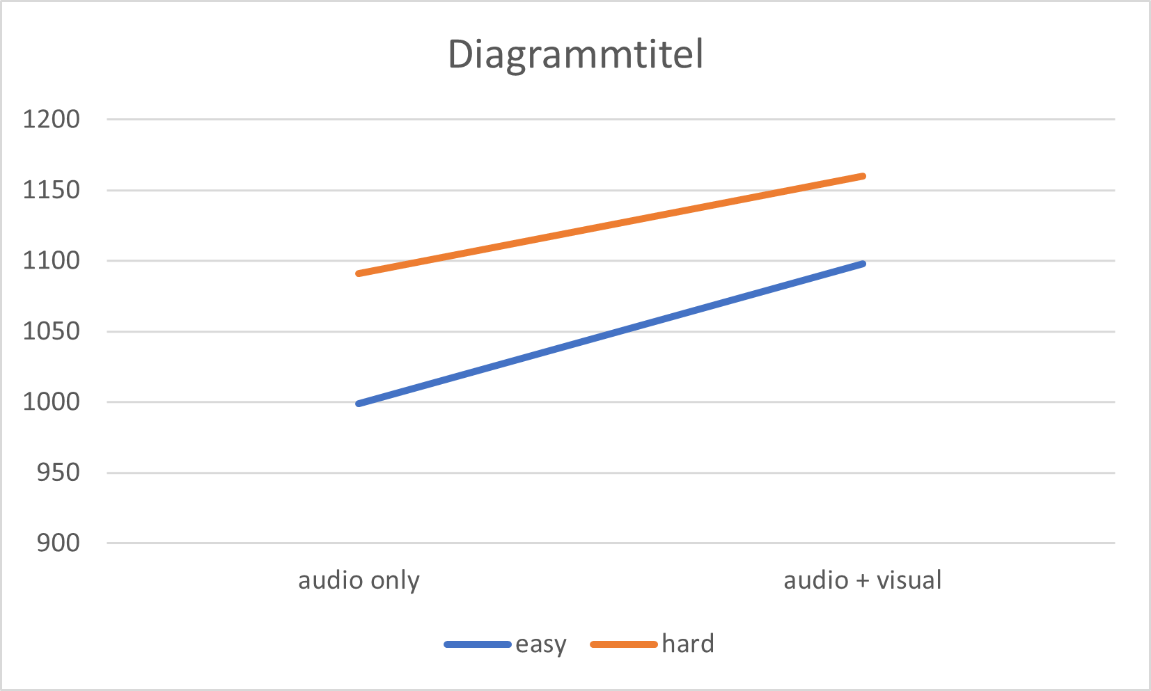

Interpretation

There is a significant interaction between modality and background noise. The negative interaction term (β = -29.53, SE = 6.755, t = -4.372, p < .001) shows that the modality slope is 29.53 ms lower (less steep) when the SNR is hard.

Three way interaction

I created a new variable that counts word length.

library(stringr)
library(psych)
library(summarytools)
library(car)

dat$stiml <- str_length(dat$stim)
freq(dat$stiml)

## Frequencies  
## dat$stiml  
## Type: Integer  
## 
##                Freq   % Valid   % Valid Cum.   % Total   % Total Cum.
## ----------- ------- --------- -------------- --------- --------------
##           3    4681     21.59          21.59     21.59          21.59
##           4   11984     55.28          76.87     55.28          76.87
##           5    4517     20.84          97.71     20.84          97.71
##           6     497      2.29         100.00      2.29         100.00
##        <NA>       0                               0.00         100.00
##       Total   21679    100.00         100.00    100.00         100.00

Hypothesis

There is a three way interaction between modality, stimgrp, and SNR

Build lm first

m5 <- lm(RT ~ modality * stiml * SNR, data = dat)
plot_model(m5, type = "pred", terms = c("modality [0,1]", "stiml [3,4,5,6]", "SNR"))

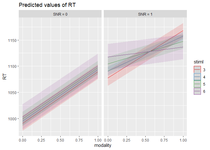
summary(m5)

## 
## Call:
## lm(formula = RT ~ modality * stiml * SNR, data = dat)
## 
## Residuals:
##     Min      1Q  Median      3Q     Max 
## -825.20 -210.69  -25.12  172.93 1387.31 
## 
## Coefficients:
##                    Estimate Std. Error t value Pr(>|t|)    
## (Intercept)        978.5426    23.6524  41.372  < 2e-16 ***
## modality            99.9038    33.1882   3.010  0.00261 ** 
## stiml                4.1322     5.7758   0.715  0.47434    
## SNR                 58.1010    34.1661   1.701  0.08904 .  
## modality:stiml      -0.3828     8.0948  -0.047  0.96228    
## modality:SNR        62.8662    47.7326   1.317  0.18784    
## stiml:SNR            9.3787     8.3364   1.125  0.26059    
## modality:stiml:SNR -23.5594    11.6379  -2.024  0.04294 *  
## ---
## Signif. codes:  0 '***' 0.001 '**' 0.01 '*' 0.05 '.' 0.1 ' ' 1
## 
## Residual standard error: 307 on 21671 degrees of freedom
## Multiple R-squared:  0.03493,    Adjusted R-squared:  0.03461 
## F-statistic:   112 on 7 and 21671 DF,  p-value: < 2.2e-16

->no sig. interaction modality:stiml; stiml:SNR, no simple effect of stiml

Random effect PID

m6 <- lmer(RT ~ 1 + modality * SNR * stiml + (1 | PID), data=dat)
plot_model(m6, type = "eff", terms = c("modality [0,1]", "stiml [3,4,5,6]", "SNR"))

## Package `effects` is not available, but needed for `ggeffect()`. Either install package `effects`, or use `ggpredict()`. Calling `ggpredict()` now.FALSE

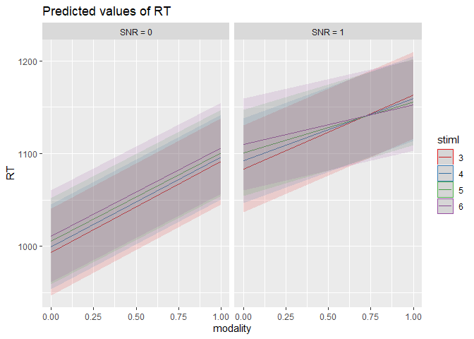
summary(m6)

## Linear mixed model fit by REML. t-tests use Satterthwaite's method [
## lmerModLmerTest]
## Formula: RT ~ 1 + modality * SNR * stiml + (1 | PID)
##    Data: dat
## 
## REML criterion at convergence: 302333
## 
## Scaled residuals: 
##     Min      1Q  Median      3Q     Max 
## -3.5897 -0.6990 -0.0254  0.5849  4.8056 
## 
## Random effects:
##  Groups   Name        Variance Std.Dev.
##  PID      (Intercept) 27952    167.2   
##  Residual             66022    256.9   
## Number of obs: 21679, groups:  PID, 53
## 
## Fixed effects:
##                     Estimate Std. Error        df t value Pr(>|t|)    
## (Intercept)          976.565     30.330   156.218  32.198  < 2e-16 ***
## modality             100.707     27.812 21619.676   3.621 0.000294 ***
## SNR                   80.741     28.620 21619.451   2.821 0.004789 ** 
## stiml                  5.751      4.838 21619.461   1.189 0.234618    
## modality:SNR          15.709     39.998 21619.614   0.393 0.694509    
## modality:stiml        -1.001      6.784 21619.716  -0.148 0.882715    
## SNR:stiml              2.964      6.983 21619.454   0.424 0.671239    
## modality:SNR:stiml   -11.313      9.753 21619.664  -1.160 0.246073    
## ---
## Signif. codes:  0 '***' 0.001 '**' 0.01 '*' 0.05 '.' 0.1 ' ' 1
## 
## Correlation of Fixed Effects:
##             (Intr) modlty SNR    stiml  md:SNR mdlty: SNR:st
## modality    -0.466                                          
## SNR         -0.452  0.493                                   
## stiml       -0.643  0.702  0.682                            
## modalty:SNR  0.324 -0.695 -0.716 -0.488                     
## modlty:stml  0.459 -0.985 -0.486 -0.714  0.685              
## SNR:stiml    0.446 -0.486 -0.985 -0.693  0.705  0.494       
## mdlty:SNR:s -0.319  0.685  0.705  0.496 -0.985 -0.696 -0.716

->no sig. interaction modality:stiml; stiml:SNR, no simple effect of stiml

Power analysis

I will follow Kumle (2021) for this (sorry). For more details see here:Link

mixedpower has advantages in computational speed and allows for more factors to be varied simultaneously compared to simr (Kumle, 2021).

Power analysis using mixedpower

#devtools::install_github("DejanDraschkow/mixedpower") # mixedpower is hosted on GitHub
library(mixedpower)

#model <- m4 # which model do we want to simulate power for?
#data <- dat # data used to fit the model
#fixed_effects <- c("RT") # all fixed effects specified in FLPmodel
#simvar <- "PID" # which random effect do we want to vary in the simulation?
#R2var <- "stim" # seconnd random effect we want to vary

# SIMULATION PARAMETERS
#steps <- c(30, 40, 50, 60, 70) # which sample sizes do we want to look at? n in sample is 53
#critical_value <- 2 # which t/z value do we want to use to test for significance?
#n_sim <- 1000 # how many single simulations should be used to estimate power?

My work pc is bad. This takes forever. I will tone down this analysis. You would use 1000 nsim. This analysis uses only one random effect. Two random effects are still possible. See documentation

Run Sim

power_FLP <- mixedpower(model = m3, data = dat,
                        fixed_effects = "modality",
                        simvar = "PID", steps = c(5,15,30),
                        critical_value = 2, n_sim = 30)

## [1] "Estimating power for step:"
## [1] 5
## [1] "Simulations for step  5  are based on  30  successful single runs"
## [1] "Estimating power for step:"
## [1] 15
## [1] "Simulations for step  15  are based on  30  successful single runs"
## [1] "Estimating power for step:"
## [1] 30
## [1] "Simulations for step  30  are based on  30  successful single runs"

power_FLP

##                  5  15 30      mode   effect
## modality 0.6333333 0.9  1 databased modality

->I guess 5 participants is too low :)

SESOI

One approach is choosing the smallest effect size of interest (SESOI)
informed decision are needed to define SESOIs in (G)LMMs. Guidance can come from previous research, literature, or practical constraints
To include a SESOI simulation, mixedpower() function can be handed a vector with SESOIs in the form of the desired beta coefficients for all specified fixed effects using the SESOI argument.
I will simply follow their recommendation to reduce all beta coefficients by 15%, however this better be derived from prior literature Fixed effect - 15%
Intercept) 1044.14 -> 887.519
modality 83.18 -> 70.703

summary(m3)

## Linear mixed model fit by REML. t-tests use Satterthwaite's method [
## lmerModLmerTest]
## Formula: RT ~ 1 + modality + (1 + modality | PID) + (1 + modality | stim)
##    Data: dat
## Control: lmerControl(optimizer = "bobyqa")
## 
## REML criterion at convergence: 302385.7
## 
## Scaled residuals: 
##     Min      1Q  Median      3Q     Max 
## -3.3646 -0.6964 -0.0140  0.5886  5.0003 
## 
## Random effects:
##  Groups   Name        Variance Std.Dev. Corr 
##  stim     (Intercept)   303.9   17.43        
##           modality      216.7   14.72   0.16 
##  PID      (Intercept) 28552.7  168.98        
##           modality     7709.8   87.81   -0.17
##  Residual             65258.8  255.46        
## Number of obs: 21679, groups:  stim, 543; PID, 53
## 
## Fixed effects:
##             Estimate Std. Error      df t value Pr(>|t|)    
## (Intercept)  1044.14      23.36   52.14  44.704  < 2e-16 ***
## modality       83.18      12.58   52.09   6.615 2.02e-08 ***
## ---
## Signif. codes:  0 '***' 0.001 '**' 0.01 '*' 0.05 '.' 0.1 ' ' 1
## 
## Correlation of Fixed Effects:
##          (Intr)
## modality -0.178

Include SESOI

SESOI <- c(887.519, 70.703) # specify SESOI
power_SESOI <- mixedpower(model = m3, data = dat,
                          fixed_effects = "modality",
                          simvar = "PID", steps = c(5,15,30),
                          critical_value = 2, n_sim = 30,
                          SESOI = SESOI, databased = T)

## [1] "Estimating power for step:"
## [1] 5
## [1] "Simulations for step  5  are based on  30  successful single runs"
## [1] "Estimating power for step:"
## [1] 15
## [1] "Simulations for step  15  are based on  30  successful single runs"
## [1] "Estimating power for step:"
## [1] 30
## [1] "Simulations for step  30  are based on  30  successful single runs"
## [1] "Estimating power for step:"
## [1] 5
## [1] "Simulations for step  5  are based on  30  successful single runs"
## [1] "Estimating power for step:"
## [1] 15
## [1] "Simulations for step  15  are based on  30  successful single runs"
## [1] "Estimating power for step:"
## [1] 30
## [1] "Simulations for step  30  are based on  30  successful single runs"

power_SESOI

##                   5        15 30      mode   effect
## modality  0.5666667 0.8666667  1 databased modality
## modality1 0.4333333 0.9333333  1     SESOI modality

multiplotPower(power_SESOI)

Power
->We see that 5 participants is too low and 15 can be pretty low as >.80 is recommended. 30 is plenty.

Navigation Structure

Load packages

Basic example

Intercept-Only Model

ICC

Add some predictors

Second example

Study design

Conditions:

Describe hypotheses

Import dataset

Screening

H1: X on Y

Outlier detection

Descriptive stats

Normality test

Define contrasts

What does this mean for later interpretations?

Visualise between participant

Define & run LMM models

Build full model

Deal with non converging models

Compare full model with nested model

Compare nested models

Bonus: to speed up likelihood-ratio tests

Investigate efects

Plot effects H1

Describe results

H2: Interaction

Define and run model

Simple effects

Interpretation

Three way interaction

Hypothesis

Build lm first

Random effect PID

Power analysis

Power analysis using mixedpower

Run Sim

SESOI

Include SESOI